What is Causal Inference? Why Do We Care? Can We Do It?
Causal inference refers to the design and analysis of data for uncovering causal relationships between treatment/intervention variables and outcome variables.
We care about causal inference because a large proportion of real-life questions of interest are questions of causality, not correlation.
Causality has been of concern since the dawn of civilization.

From: Mesopotamiske farmakopéer, accessed September 26, 2014.
Rigorous statistical frameworks for causality that can be applied to many types of data have been established for only a century.

The Fall 2021 Distinguished Theme Seminar Series will have talks by major figures in causal inference, including Donald B. Rubin, Judea Pearl, and James M. Robins.
Example: The Causal Effect of Smoking
There is a wide consensus that smoking is bad for humans. But what is the basis for this consensus?
Experiments on smoking cannot be performed on humans due to medical ethics.
There exist significant observational data on human smoking, in which no controls are placed over how smoking is assigned to the subjects. What inferences do we obtain from such observational studies?
Cochran (1968: p. 297) gives three observational studies on smoking: a six-year Canadian study, a five-year British study, and a 20-month U.S.A. study.
The outcomes in these studies are summarized by the death rates per 1000 person-years, defined as
$$ \frac{\text{Total # of Deaths}}{\text{Total # of Person-Year Exposures}} \times 10^3. $$| Smoking Group | Canadian | British | U.S.A. |
|---|---|---|---|
| Non-smokers | 20.2 | 11.3 | 13.5 |
| Cigarettes only | 20.5 | 14.1 | 13.5 |
| Cigars and/or pipe | 35.5 | 20.7 | 17.4 |
🤔 From these studies, it appears that cigar/pipe smokers should instead just smoke cigarettes. Is that reasonable? What else can be lurking behind the scenes?
| Smoking Group | Canadian Mean Age | British Mean Age | U.S.A. Mean Age |
|---|---|---|---|
| Non-smokers | 54.9 | 49.1 | 57.0 |
| Cigarettes only | 50.5 | 49.8 | 53.2 |
| Cigars and/or pipe | 65.9 | 55.7 | 59.7 |
💡 Cigar/pipe smokers are older! That can explain (in part) their higher death rate.
💡 Cigarette smokers are fairly young in this dataset, and so likely did not develop any smoking-related diseases during the time period of their respective studies.
Confounding exists in these studies: cigar smokers are more likely to be older than other subjects, and hence more likely to die. Standard analyses cannot disentangle these two in the observational study!
Example: What Have We Learned?
Systematic differences in pre-treatment variables/covariates for subjects assigned different treatments confound inferences and introduce bias.
Confounding means a difference between the treatment groups, other than the treatments, related to the response (Freedman, 2009: p. 2).
Carefully designed experiments are the gold standard for causal inference because they can minimize bias from confounding (among other problems), and enable inferences with minimal assumptions.
Cochran (1965, 1968), Rubin (1973): Observational studies can be designed so as to reduce biases due to confounding, and yield valid causal inferences.
So Why Care About Causal Inference? And Can We Do It?
The typical goals in scientific investigations are to identify
- factors that affect a response, and
- details of these causal relationships.
Designed experiments are the gold standard for causal inference because the controls and physical act of randomization in experiments guarantee, in expectation, no bias due to confounding, and methods for statistical analyses that require no parametric assumptions (Imbens & Rubin, 2015).
Observational studies can yield valid causal inferences if they are designed prior to analysis, so as to approximate a randomized experiment.
Epiphanies of Fisher and Neyman
Fisherian Randomization-Based Tests and Intervals
To evaluate the claim that treatment differs from control, we construct a reference distribution for a test statistic.
The test statistic captures the difference between treatment and control outcomes in the observed data.
The reference distribution represents a characteristic set of outcomes that would be realized if treatment was without effect (i.e., under the null).
The observed test statistic is compared to the reference distribution, and if found to be extreme the result is called statistically significant.
Fisher's genius (1925, 1935): For randomized experiments, the combination of the physical act of randomization with a sharp null hypothesis enables the construction of a reference distribution for testing the hypothesis that treatment is entirely without effect.
Fisher's approach is referred to as a Fisherian randomization test for a sharp null hypothesis.
It can be performed for all randomized experiments, not just CRDs.
Fisherian randomization tests can be extended to construct intervals for additive treatment effects (Pitman, 1937, 1938; Imbens & Rubin, 2015, p. 64).
Example: Evaluating a Job Training Program (LaLonde, 1986)
Experimental Units
$445$ men in 1976.
☝ An experimental unit is a physical object at a particular point in time.
Covariates
Age, years of education, ethnicity, etc.
Treatment Factor
Activity, with two levels: job training (1) or nothing (0).
Potential Outcome
Annual earnings in 1978 (in dollars).
Assignment Mechanism
CRD with $185$ treated units ($N_1 = 185, N_0 = 260$).
Question of Interest
Is there any causal effect of the job training program?
What is the causal effect of the job training program?
General Procedure for the Fisherian Randomization Test
Specify the test statistic (what effect do we care about measuring?).
Specify the sharp null hypothesis (what does it mean to be "entirely without effect"?).
Specify the direction of extremeness and significance level $\alpha$ (what does it mean to be "extreme"?).
Calculate observed test statistic $T^{\mathrm{obs}}$.
Impute missing outcomes under the sharp null (more to come!).
For each possible treatment assignment vector, calculate the value of the test statistic $T$ that would have been observed under that assignment.
Calculate the $p$-value for the observed test statistic as $p = \mathrm{Pr}(T \geq T^{\mathrm{obs}})$.
Decide to reject or fail to reject the sharp null hypothesis $(p \leq \alpha, p > \alpha)$.
Example: Fisherian Randomization Tests for the LaLonde Data
We proceed to perform the Fisherian randomization test for the LaLonde data via Monte Carlo approximation.
The first test statistic that we consider is the absolute difference in averages.
Lalonde_data = read.table("LaLonde_experiment_data.txt", header=T, sep=" ")
Lalonde_data = Lalonde_data[,c(2,1)]

observed_test_statistic = abs(mean(Lalonde_data[Lalonde_data[,1]==1,2]) -
                              mean(Lalonde_data[Lalonde_data[,1]==0,2]))

number_of_Monte_Carlo_draws = 10^5

observed_imputed_outcomes = matrix(NA, nrow=nrow(Lalonde_data), ncol=2)
observed_imputed_outcomes[,1] = Lalonde_data[,2]
observed_imputed_outcomes[,2] = Lalonde_data[,2]

test_statistics = rep(NA, number_of_Monte_Carlo_draws)

progress_bar = txtProgressBar(min=1, max=number_of_Monte_Carlo_draws, style = 3)

for(i in 1:number_of_Monte_Carlo_draws)
{
  possible_assignment = sample(Lalonde_data[,1], replace=F)
  test_statistics[i] = abs(mean(observed_imputed_outcomes[possible_assignment==1,2]) -
                           mean(observed_imputed_outcomes[possible_assignment==0,1]))
  setTxtProgressBar(progress_bar, i)
}
close(progress_bar)

p_value = mean(test_statistics>=observed_test_statistic)

hist(test_statistics, breaks=50,
     xlab=expression(paste("T(W, "*y^obs*")")),
     main="Reference Distribution for LaLonde Data", freq=FALSE)
abline(v=observed_test_statistic, lty=2, lwd=2)
text(2200,8e-4, expression(paste(T^obs*" = 1794.341")))
cat("The p-value for this test is:", p_value, fill=TRUE)

We next perform the Fisherian randomization test using the t-test statistic.
observed_test_statistic = (mean(Lalonde_data[Lalonde_data[,1]==1,2]) -
                           mean(Lalonde_data[Lalonde_data[,1]==0,2]))/
                          sqrt(var(Lalonde_data[Lalonde_data[,1]==1,2])/sum(Lalonde_data[,1]==1) +
                               var(Lalonde_data[Lalonde_data[,1]==0,2])/sum(Lalonde_data[,1]==0))
number_of_Monte_Carlo_draws = 10^5

observed_imputed_outcomes = matrix(NA, nrow=nrow(Lalonde_data), ncol=2)
observed_imputed_outcomes[,1] = Lalonde_data[,2]
observed_imputed_outcomes[,2] = Lalonde_data[,2]

test_statistics = rep(NA, number_of_Monte_Carlo_draws)

progress_bar = txtProgressBar(min=1, max=number_of_Monte_Carlo_draws, style = 3)

for(i in 1:number_of_Monte_Carlo_draws)
{
  possible_assignment = sample(Lalonde_data[,1], replace=F)
  test_statistics[i] = (mean(observed_imputed_outcomes[possible_assignment==1,2]) -
                        mean(observed_imputed_outcomes[possible_assignment==0,1]))/
                       sqrt(var(observed_imputed_outcomes[possible_assignment==1,2])/185 +
                            var((observed_imputed_outcomes[possible_assignment==0,1])/260))
  setTxtProgressBar(progress_bar, i)
}
close(progress_bar)

p_value = 2*min(mean(test_statistics>=observed_test_statistic),
                mean(test_statistics<=observed_test_statistic))

hist(test_statistics, breaks=50,
     xlab=expression(paste("T(W, "*y^obs*")")),
     main="Reference Distribution for t-Test Statistic for LaLonde Data",
     freq=FALSE)
abline(v=observed_test_statistic, lty=2, lwd=2)
text(3.8,0.3, expression(paste(T^obs*" = 2.67")))
cat("The p-value for this test is:", p_value, fill=TRUE)

Fisherian/Fiducial Intervals for Treatment Effects
Let $Y_i(0)$ denote the outcome for experimental unit $i$ when it is given control, and $Y_i(1)$ the outcome for experimental unit $i$ when it is given treatment.
Fisher's sharp null hypothesis can be written as:
$$ H_0^{\#}: Y_i(0) = Y_i(1) \ \mathrm{for \ all} \ i = 1, \ldots, N. $$We don't have to believe Fisher's sharp null, but we may wish to see how strongly the data speak against it.
We could also test sharp null hypotheses on constant additive treatment effects.
$$ H_{0,(c)}^{\#}: Y_i(0) + c = Y_i(1) \ \mathrm{for \ all} \ i = 1, \ldots, N $$Fisherian randomization tests for a set $\mathcal{C}$ of $c$ values enable the construction of an interval for the constant additive treatment effect.
Such a Fisherian/Fiducial interval (Pitman, 1937, 1938; Imbens & Rubin, 2015, p. 64) is arguably more informative than a single Fisherian randomization test for $H_0^{\#}$.
General Procedure for the Fisherian/Fiducial Interval for a Constant Additive Treatment Effect
Specify the test statistic for the Fisherian randomization test.
Specify a set of constant additive treatment effects $\mathcal{C} \subset \mathbb{R}$.
Specify the direction of extremeness and significance level $\alpha$ for the Fisherian randomization test.
Let $\mathcal{I}$ denote the empty set.
For each $c \in \mathcal{C}$:
Perform a Fisherian randomization test for the sharp null hypothesis
$$ H_{0,(c)}^{\#}: Y_i(0) + c = Y_i(1). $$
If $H_{0,(c)}^{\#}$ fails to be rejected at the $\alpha$ significance level, include $c$ in $\mathcal{I}$ (i.e., update $\mathcal{I}$ according to $\mathcal{I} \leftarrow \mathcal{I} \cup \{c\}$ as in R notation).
Return $\mathcal{I}$ as the $100(1-\alpha)\%$ Fisherian/Fiducial interval.
Properties of Fisherian/Fiducial Intervals for Constant Additive Treatment Effects
In the case of a constant additive treatment effect (i.e., $Y_i(0) + c = Y_i(1)$ for all $i = 1, \ldots, N$), the $100(1-\alpha)\%$ Fisherian/Fiducial interval is a $100(1-\alpha)\%$ confidence interval with respect to the probability distribution induced by the assignment mechanism.
Furthermore, in this case the $100(1-\alpha)\%$ Fisherian/Fiducial interval is a $100(1-\alpha)\%$ confidence interval for the average treatment effect $\bar{Y}(1) - \bar{Y}(0)$.
Example: 95$\mathbf{\%}$ Fisherian/Fiducial Interval for the LaLonde Data
An effective approach to construct the $95\%$ Fisherian/Fiducial interval is to perform Fisherian randomization tests so as to identify the lower and upper bounds of the interval.
number_of_Monte_Carlo_draws = 10^5

random_assignment_vectors = matrix(rep(NA, (number_of_Monte_Carlo_draws*nrow(Lalonde_data))),
                                   nrow=nrow(Lalonde_data), ncol=number_of_Monte_Carlo_draws)

for(i in 1:number_of_Monte_Carlo_draws)
{
  random_assignment_vectors[,i] = sample(Lalonde_data[,1], replace=FALSE)
}


Fisher_p_values = function(data, treatment_indicators, lowerBound, upperBound, spacing,
                           matrix_of_random_assignment_vectors)
{
  observed_test_statistic = mean(data[treatment_indicators==1]) -
                            mean(data[treatment_indicators==0])

  observed_imputed_outcomes = cbind(rep(NA, length(data)), rep(NA, length(data)))
  possible_effects = seq(lowerBound, upperBound, spacing)

  progress_bar = txtProgressBar(min=1, max=length(possible_effects), style = 3)

  for(j in 1:length(possible_effects))
  {
    for(k in 1:length(data))
    {
      if(treatment_indicators[k]==0)
      {
        observed_imputed_outcomes[k,1] = data[k]
        observed_imputed_outcomes[k,2] = observed_imputed_outcomes[k,1] + possible_effects[j]
      }

      if(treatment_indicators[k]==1)
      {
        observed_imputed_outcomes[k,2] = data[k]
        observed_imputed_outcomes[k,1] = observed_imputed_outcomes[k,2] - possible_effects[j]
      }
    }

    reference_distribution = rep(NA, ncol(matrix_of_random_assignment_vectors))

    for(i in 1:ncol(matrix_of_random_assignment_vectors))
    {
      reference_distribution[i] = mean(observed_imputed_outcomes[matrix_of_random_assignment_vectors[,i]==1,2])-
                                  mean(observed_imputed_outcomes[matrix_of_random_assignment_vectors[,i]==0,1])
    }

    p_value = 2*min(c(mean(reference_distribution>=observed_test_statistic),
                      mean(reference_distribution<=observed_test_statistic)))

    setTxtProgressBar(progress_bar, j)
    cat("", fill=TRUE)
    cat("The p-value for ",possible_effects[j]," is ", p_value, fill=TRUE)
  }

  close(progress_bar)
}
By trial and error, we recognize that the lower bound of the interval is approximately 535.
Fisher_p_values(Lalonde_data[,2], Lalonde_data[,1], 535, 536, 0.1, random_assignment_vectors)
In addition, we recognize that the upper bound of the interval is approximately 3015.
Fisher_p_values(Lalonde_data[,2], Lalonde_data[,1], 3014, 3015, 0.1, random_assignment_vectors)
Thus, the $95\%$ Fisherian/Fiducial interval for the constant additive treatment effect is approximately (535, 3015).
Neymanian Randomization-Based Estimation and Intervals
Neyman's genius (1923):
- Concepts and notations for potential outcomes and causal estimands.
| Unit | $X_i$ | $Y_i(0)$ | $Y_i(1)$ |
|---|---|---|---|
| 1 | $X_1$ | $Y_1(0)$ | $Y_1(1)$ |
| 2 | $X_2$ | $Y_2(0)$ | $Y_2(1)$ |
| $\vdots$ | $\vdots$ | $\vdots$ | $\vdots$ |
| $N$ | $X_N$ | $Y_N(0)$ | $Y_N(1)$ |
☝ We are assuming no hidden variations in the treatments, and that the experimental units do not interfere with one another. This is also known as the Stable Unit-Treatment Value Assumption (SUTVA, Imbens & Rubin, 2015: p. 10).
Finite-population causal estimand: Comparison of potential outcomes for one set of experimental units.
$$ \left \{ Y_i(\mathrm{1}) : i = 1, \ldots, N \right \} \ \mathrm{vs.} \ \left \{ Y_i(\mathrm{0}) : i = 1, \ldots, N \right \} $$The choice of estimand is typically governed by the question of interest.
For example, in the previous table, one causal estimand is the average treatment effect:
$$\tau = \bar{Y}(1) - \bar{Y}(0) = \frac{1}{N} \sum_{i=1}^N Y_i(1) - \frac{1}{N} \sum_{i=1}^N Y_i(0).$$☝ A causal effect is not defined in terms of comparisons of outcomes at different times, as in before-after comparisons.
- Knowledge of the assignment mechanism is sufficient to evaluate properties of estimators of causal estimands.
| Unit | $X_i$ | Control (0) or Treatment (1)? | $Y_i(0)$ | $Y_i(1)$ | $Y_i(1) - Y_i(0)$ |
|---|---|---|---|---|---|
| 1 | $X_1$ | 1 | ? | ✔ | ? |
| 2 | $X_2$ | 0 | ✔ | ? | ? |
| $\vdots$ | $\vdots$ | $\vdots$ | $\vdots$ | $\vdots$ | $\vdots$ |
| $N$ | $X_N$ | 1 | ? | ✔ | ? |
We never observe all potential outcomes or all unit-level effects.
Causal inference is a missing data problem, and a key role is played by the assignment mechanism.
Assignment mechanism: Description of how treatments are assigned to the experimental units (and the corresponding outcomes are observed).
Observed outcomes can possibly help us infer causal effects only when we account for how units came to receive their treatments.
☝ Potential outcomes and causal effects are well-defined regardless of the assignment mechanism.
Treatment Assignment Indicators, Observed Outcomes, and Estimators
$W_i$: treatment assignment indicator for unit $i$.
$$ W_i = \begin{cases} 1 & \mbox{if unit} \ i \ \mbox{is assigned treatment,} \\ 0 & \mbox{if unit} \ i \ \mbox{is assigned control}. \end{cases} $$Observed outcomes are functions of potential outcomes and treatment assignment indicators.
$$ y_i^{\mathrm{obs}} = W_iY_i(1) + (1-W_i)Y_i(0) $$$$ y_i^{\mathrm{mis}} = (1-W_i)Y_i(1) + W_iY_i(0) $$☝ Potential outcomes and causal effects are well-defined regardless of treatment assignment indicators.
⚠ Do not confuse potential outcomes with observed outcomes!
Estimator of $\tau = \bar{Y}(1) - \bar{Y}(0)$: $$ \hat{\tau} = \bar{y}^{\mathrm{obs}}(1) - \bar{y}^{\mathrm{obs}}(0) = \frac{1}{N_1}\sum_{i=1}^N W_i Y_i(1) - \frac{1}{N_0}\sum_{i=1}^N (1-W_i)Y_i(0)$$.
Neyman (1923) considered
bias of $\hat{\tau}$ for estimation of $\tau$,
estimation of $\mathrm{Var}(\hat{\tau})$, and
interval estimation for $\tau$.
Definition of Expectation and Unbiased Estimation
The expectation of an estimator $\hat{\tau}$ is
$$ \mathbb{E}(\hat{\tau}) = \sum_{\mathbf{w} \in \{0,1\}^N} \hat{\tau}(\mathbf{w}, \mathbf{y}^{\mathrm{obs}}, \mathbf{X}) \mathrm{Pr}(\mathbf{W} = \mathbf{w}). $$The bias of $\hat{\tau}$ is $\mathbb{E}(\hat{\tau}) - \tau$.
An estimator $\hat{\tau}$ is unbiased for $\tau$ if $\mathbb{E}(\hat{\tau}) = \tau$.
Proof: $\mathbb{E}(\hat{\tau}) = \tau$ for a Completely Randomized Design (CRD)
Consider a CRD with $0 < N_1 < N$.
\begin{align*} \mathbb{E}(\hat{\tau}) &= \mathbb{E} \left \{ \bar{y}^{\mathrm{obs}}(1) - \bar{y}^{\mathrm{obs}}(0) \right \} \\ &= \mathbb{E} \left \{ \frac{1}{N_1}\sum_{i=1}^N W_iY_i(1) - \frac{1}{N_0}\sum_{i=1}^N(1-W_i)Y_i(0) \right \} \\ &= \frac{1}{N_1} \sum_{i=1}^N \mathbb{E} \{ W_i Y_i(1) \} - \frac{1}{N_0}\sum_{i=1}^N \mathbb{E}\{ (1-W_i) Y_i(0) \} \\ &= \frac{1}{N_1} \sum_{i=1}^N \mathbb{E} (W_i) Y_i(1) - \frac{1}{N_0}\sum_{i=1}^N \mathbb{E}(1-W_i) Y_i(0) \\ &= \frac{1}{N_1} \sum_{i=1}^N \left ( \frac{N_1}{N} \right ) Y_i(1) - \frac{1}{N_0}\sum_{i=1}^N \left ( \frac{N_0}{N} \right ) Y_i(0) \\ &= \bar{Y}(1) - \bar{Y}(0) \end{align*}In a CRD, the observed difference in means is an unbiased estimator of the finite-population average treatment effect.
☝ No model on the potential outcomes is required for this conclusion. All that is required is the distribution on $\mathbf{W}$, which is the assignment mechanism.
Example: Estimation of $\tau$ for the LaLonde Data
ATE_estimate = mean(Lalonde_data[Lalonde_data[,1]==1,2]) - mean(Lalonde_data[Lalonde_data[,1]==0,2])

cat("The point estimator of the average treatment effect is:", ATE_estimate, fill=TRUE)
Neyman's Next Step: Calculation of Var$(\hat{\tau})$
\begin{align*} \mathrm{Var}(\hat{\tau}) &= \mathrm{Var} \left \{ \bar{y}^{\mathrm{obs}}(1) - \bar{y}^{\mathrm{obs}}(0) \right \} \\ &= \mathrm{Var} \left \{ \frac{1}{N_1} \sum_{i=1}^N W_i Y_i(1) - \frac{1}{N_0} \sum_{i=1}^N (1-W_i)Y_i(0) \right \} \end{align*}Note the value of Cov$(W_i, W_j)$ for distinct $i, j \in \{1, \ldots, N\}$ in a CRD.
Calculation of Var$(\hat{\tau})$ involves some algebra, and the details can be found in (Imbens \& Rubin, 2015: p. 87 - 89).
After some algebra, we have that in a CRD with $0 < N_1 < N$, for $\hat{\tau} = \bar{y}^{\mathrm{obs}}(1) - \bar{y}^{\mathrm{obs}}(0)$, $$ \mathrm{Var}(\hat{\tau}) = \frac{S_1^2}{N_1} + \frac{S_0^2}{N_0} - \frac{S_{10}^2}{N}, $$ where $$ S_1^2 = \frac{1}{N-1}\sum_{i=1}^N \left \{Y_i(1) - \bar{Y}(1) \right \}^2, $$ $$ S_0^2 = \frac{1}{N-1}\sum_{i=1}^N \left \{Y_i(0) - \bar{Y}(0) \right \}^2, \ \mathrm{and} $$ $$ S_{10}^2 = \frac{1}{N-1}\sum_{i=1}^N \left [ \{Y_i(1) - Y_i(0) \} - \{ \bar{Y}(1) - \bar{Y}(0) \} \right ]^2. $$
$S_1^2$: Finite-population variance of the treatment potential outcomes.
$S_0^2$: Finite-population variance of the control potential outcomes.
$S_{10}^2$: Finite-population variance of the unit-level causal effects. This term is also related to the correlation between treatment and control potential outcomes (Imbens & Rubin, 2015: p. 90 - 91).
Neyman's (1923) Biased Estimator for Var$(\hat{\tau})$
An unbiased estimator of $S_1^2/N_1$ is $s_1^2/N_1$, where $$ s_1^2 = \frac{1}{N_1 - 1}\sum_{i: W_i^{\mathrm{obs}} = 1} \left \{ y_i^{\mathrm{obs}} - \bar{y}^{\mathrm{obs}}(1) \right \}^2. $$
An unbiased estimator of $S_0^2/N_0$ is $s_0^2/N_0$, where $$ s_0^2 = \frac{1}{N_0 - 1}\sum_{i: W_i^{\mathrm{obs}} = 0} \left \{ y_i^{\mathrm{obs}} - \bar{y}^{\mathrm{obs}}(0) \right \}^2. $$
⚠ An unbiased estimator of $S_{10}^2/N$ does not exist!
We can never see both potential outcomes simultaneously for any experimental unit.
We cannot infer the correlation between the potential outcomes based only on the observed outcomes.
Neyman (1923): Estimate $V = \mathrm{Var}(\hat{\tau})$ by $\hat{V} = s_1^2/N_1 + s_0^2/N_0$.
$\mathbb{E}(\hat{V}) \geq V$.
If $Y_i(1) - Y_i(0) = c$ for all $i = 1, \ldots, N$, then $\mathbb{E}(\hat{V}) = V$.
- 🤔 Why is this true?
We typically use this biased estimator of Var$(\hat{\tau})$ because it provides "conservative" inferences for $\tau$.
If our sample of units is randomly chosen from a larger population, bias in the variance estimator is no longer an issue (Imbens \& Rubin, 2015: p. 98 - 101).
Example: Estimation of Var$(\hat{\tau})$ for the LaLonde Data
var_estimate = var(Lalonde_data[Lalonde_data[,1]==1,2])/sum(Lalonde_data[,1]==1) +
               var(Lalonde_data[Lalonde_data[,1]==0,2])/sum(Lalonde_data[,1]==0)

cat("The point estimator of the variance of the treatment effect is:", var_estimate, fill=TRUE)
Neyman's (1923) Interval Estimator for $\tau$
Armed with $\hat{\tau}$ and $\hat{V}$, Neyman (1923) finally constructed a $(1 - \alpha) \%$ interval estimator for $\tau$ as $$ \hat{\tau} \pm z_{\alpha/2} \sqrt{\hat{V}}. $$
As $\hat{V}$ is an upwardly biased estimator of Var$(\hat{\tau})$, this interval estimator will have coverage probability greater than $1 - \alpha$.
This is why Neyman (1934) defined a $(1 - \alpha) \%$ confidence interval to have coverage probability at least $1 - \alpha$, not exactly $1 - \alpha$.
Example: $95 \%$ Interval for $\tau$ for the Lalonde Data
CI = ATE_estimate + c(-1,1)*1.96*sqrt(var_estimate)

cat("The 95% Neyman interval for the treatment effect is:", CI, fill=TRUE)
Summary of Epiphanies
Knowledge of the treatment assignment mechanism can facilitate valid statistical inferences, such as
hypothesis testing,
point estimation, and
interval estimation.
Advantages of the physical act of randomization are that it
reduces the influence of subjective bias in treatment assignments, and
protects against latent variables or "lurking variables" (in expectation).
The consideration of potential outcomes enable one to specify a consistent definition of a causal estimand, i.e., one that does not change depending on the method of analysis for the observed data. Accordingly, causal inferences obtained from different analytical approaches can be directly compared. Also, one does not have to specify a causal estimand in terms of parameters in a model or machine learning algorithm.
The Neyman-Fisher Controversy of 1935
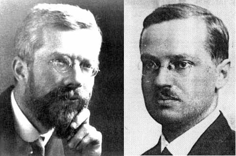
The Neyman-Fisher controversy of 1935 arose in part because Neyman sought to determine whether Fisher's ANOVA F-test for the randomized complete block and Latin square designs would still be valid when testing Neyman's more general null hypothesis that was formulated using potential outcomes.
Unfortunately, Neyman's calculations and general reasoning were incorrect (Sabbaghi and Rubin, 2014).
This controversy had many unfortunate consequences.
Hostile relationship between Neyman and Fisher, with each seeking to undermine the other.
Fisher avoided potential outcomes, leading him to make certain oversights in causal inference (Rubin, 2005).
- Never bridged his works on experimental design and parametric modeling.
- Gave generally flawed advice on the analysis of covariance to adjust for posttreatment concomitants in randomized trials.
More effort was devoted to issues in randomization, especially regarding error estimation (Cox, 2012).
Undue emphasis on linear models for observed outcomes.
- Motivation for Box-Cox transformation.
- Lindley and Novick: randomization not necessary, but useful (Lindley \& Novick, 1981).
What was lost: explicit randomization, as extolled by Fisher, provides the scientist with internally consistent statistical inferences that require no standard modeling assumptions, such as those required for linear regression.
🙃 Many textbooks on experimental design focus solely on Normal theory linear models, without realizing that such models were originally motivated in the past as approximations for randomization inference.
Model assumptions should be driven by Science, not by seemingly necessary requirements for classical procedures to have desired properties.
🙃 Two of the greatest statisticians argued over incorrect calculations and inexact measures of unbiasedness.
"Yet after this long journey, I feel that it is a pity that so much valuable time should be given to unfriendly criticism, based on mis-statements and errors and, subsequently, to the necessary corrections." (Neyman, 1935)
Future Directions in Causal Inference
There are many areas of ongoing research in causal inference.
Bridging the gap between modern experimental design and causal inference.
Addressing violations of SUTVA.
Machine learning for causal effects.
Transfer learning.
Synthetic controls.
Case-control studies.
Bridging the Gap Between Modern Experimental Design and Causal Inference
Modern experimental design is characterized by more sophisticated treatment and blocking structures than those observed in existing causal inference problems.
Highly fractionated, non-regular designs.
Optimum designs.
Robust parameter designs.
Computer experiments
Complicated hierarchical/nesting structures.
A great deal of work can be done to explore the foundations and fundamentals of modern designs for causal inference.
Addressing Violations of SUTVA
An active area of research is performing causal inference under interference, specifically, when network or peer effects exist.
Transfer Learning
Standard methods for causal inference enable internally valid inferences on treatment effects in a finite-population.
A novel area of causal inference research is focused on enabling externally valid inferences on treatment effects.
Synthetic Controls
A problem that can arise in observational studies is that the control group is not sufficiently large in size to enable satisfactory matching or subclassification.
In such cases, a novel solution is to simulate synthetic controls that match the observed treated units.
Case-Control Studies
Case-control studies are common in epidemiology.
Existing logistic regression-based methods in case-control studies may not yield valid causal conclusions.
Furthermore, they do not permit outcome-free design, which is a hallmark of the design and analysis of observational studies under the Rubin Causal Model.
Supplement: Regularity Assumptions for the Assignment Mechanism, and the Propensity Score
The assignment mechanism is a description of the probability of any vector of assignments for the entire population.
Assignment mechanism: $\mathrm{Pr}\{\mathbf{W} \mid \mathbf{X}, \mathbf{Y}(0), \mathbf{Y}(1) \}$.
☝ $\displaystyle \sum_{\mathbf{w} \in \{0,1\}^N} \mathrm{Pr}\{\mathbf{W} = \mathbf{w} \mid \mathbf{X}, \mathbf{Y}(0), \mathbf{Y}(1) \} = 1$ (Imbens & Rubin, 2015: p. 34).
Unit-level assignment probability for unit $i$: $p_i(\mathbf{X}, \mathbf{Y}(0), \mathbf{Y}(1)) = \displaystyle \sum_{\mathbf{w}: w_i = 1} \mathrm{Pr}\{\mathbf{W} = \mathbf{w} \mid \mathbf{X}, \mathbf{Y}(0), \mathbf{Y}(1) \}$.
Individualistic Assignment
There exists a function $q: \mathbb{R}^{K+2} \rightarrow (0,1)$ such that for all subjects $i$, $$ p_i(\mathbf{X}, \mathbf{Y}(0), \mathbf{Y}(1)) = q(X_i, Y_i(0), Y_i(1)) $$ and $$\mathrm{Pr} \{ \mathbf{W} \mid \mathbf{X}, \mathbf{Y}(0), \mathbf{Y}(1) \} = c \displaystyle \prod_{i=1}^N q(X_i, Y_i(0), Y_i(1))^{W_i}\{1-q(X_i,Y_i(0),Y_i(1))\}^{1-W_i} $$ for some set of $(\mathbf{W}, \mathbf{X}, \mathbf{Y}(0), \mathbf{Y}(1))$, where $c$ is the normalization constant for the probability mass function of the treatment assignment mechanism.
💡 If an assignment mechanism is not individualistic, then some subjects' treatment assignments would depend on the covariates and potential outcomes of other subjects, which would complicate the design and analysis of experiments or observational studies.
☝ Besides sequential experiments (such as multi-armed bandits), the individualistic assignment mechanism is not particularly controversial.
Probabilistic Assignment
For all subjects $i$, $0 < p_i(\mathbf{X}, \mathbf{Y}(0), \mathbf{Y}(1)) < 1$.
💡 A probabilistic assignment mechanism permits the consideration of all subjects for the design and analysis of an experiment or observational study, and reduces the risk of extrapolation biases when estimating treatment effects.
☝ If an experimental unit receives treatment with either probability zero or probability one, then estimates of the treatment effect for similar such experimental units will necessarily involve extrapolation, and so such units should not be considered for causal inferences. The probabilistic assignment mechanism is thus intuitive and justifiable.
Unconfounded Assignment
For any $\mathbf{w} \in \{0, 1\}^N$ and potential outcome vectors $\mathbf{Y}(0), \mathbf{Y}'(0), \mathbf{Y}(1), \mathbf{Y}'(1) \in \mathbb{R}^N$, $ \mathrm{Pr} \{ \mathbf{W} = \mathbf{w} \mid \mathbf{X}, \mathbf{Y}(0), \mathbf{Y}(1) \} = \mathrm{Pr} \{ \mathbf{W} = \mathbf{w} \mid \mathbf{X}, \mathbf{Y}'(0), \mathbf{Y}'(1) \}. $$
💡 No lurking confounders! The observed covariates contain all the information governing treatment assignment, and no additional variables associated with the outcomes are related to treatment assignment.
☝ The unconfoundedness assumption is perhaps the most controversial assumption for causal inference on observational studies under the Rubin Causal Model. Having said that, it is commonly invoked across a wide range of domains (Imbens & Rubin, 2015: p. 262 - 263).
Regular assignment mechanism/Strongly ignorable treatment assignment: Combination of the individualistic, probabilistic, and unconfounded assignment assumptions.
💡 A regular assignment mechanism justifies designing an observational study so as to compare treated and control subjects with the same covariates for inferring causal effects.
If a treated and control subject have the same covariates, then their treatment assignments have effectively been performed according to some random mechanism.
Comparing treated and control subjects with the same covariates should thus yield unbiased inferences for the treatment effects in the designed observational study.
💡 If an (unknown) assignment mechanism is regular, then for that assignment mechanism we have that
a completely randomized design was effectively conducted for subpopulations of experimental units with the same covariates, and that
a causal interpretation can be attached to the comparison of observed outcomes for treated and control units within the subpopulations.
The second implication holds because the observed outcomes within a particular subpopulation constitute a random sample of the potential outcomes for that subpopulation, so that the difference in observed averages is unbiased for the subpopulation average treatment effect.
💡 The fact that the assignment mechanism is unknown does not matter for this result.
These desirable implications of a regular assignment mechanism can be operationalized for deriving valid, unbiased causal inferences from observational studies that have regular assignment mechanisms by means of the propensity scores.
Propensity score for a regular assignment mechanism: Unit-level assignment probability, typically denoted by the function $e: \mathbb{R}^K \rightarrow (0,1)$.
Supplement: The Importance and Controversy of Unconfoundedness
The unconfoundeness assumption is critical to the utility of regular assignment mechanisms.
For an assignment mechanism to be unconfounded, we must have a sufficiently rich set of covariates such that adjusting for differences in their observed values between the treatment and control groups will remove systematic biases in the causal inferences.
The unconfoundness assumption is typically the most controversial assumption for causal inferences on observational studies under the Rubin Causal Model.
Furthermore, this assumption is not testable: the data are not directly informative about the distribution of $Y_i(0)$ for those units $i$ given treatment, nor are they directly informative about the distribution of $Y_j(1)$ for those units $j$ given control.
Our inability to test unconfoundedness in general is similar to our inability to test whether a missing data mechanism is missing not at random (MNAR) or missing at random (MAR).
As unconfoundedness is such an important and controversial assumption, supplementary analyses that can assess its plausibility can be important for drawing causal conclusions.
References
Cochran W.G. (1965). The planning of observational studies of human populations. Journal of the Royal Statistical Society: Series A, 128(2), 234-255.
Cochran W.G. (1968). The effectiveness of adjustment by subclassification in removing bias in observational studies. Biometrics, 24(2), 295-313.
Cox D.R. (2012). Statistical causality: some historical remarks. In C. Berzuini, P. Dawid, and L. Bernardinelli (eds.), Causality: Statistical Perspectives and Applications, Wiley Series in Probability and Statistics, pp. 1-5. Wiley.
Fisher R.A. (1925). Statistical Methods for Research Workers, Oliver and Boyd (1st edition).
Fisher R.A. (1935). Design of Experiments, Oliver and Boyd (1st edition).
Freedman D.A. (2009). Statistical Models: Theory and Practice, Cambridge University Press (2nd edition).
Imbens G.W. and D.B. Rubin (2015). Causal Inference for Statistics, Social, and Biomedical Sciences: An Introduction, Cambridge University Press (1st edition).
LaLonde R.J. (1986). Evaluating the econometric evaluations of training programs with experimental data. The American Economic Review 76(4), 604-620.
Little R.J.A. and Rubin D.B. (2002). Statistical Analysis With Missing Data. Wiley-Interscience (2nd edition).
Lindley D.V. and Novick M.R. (1981). The role of exchangeability in inference. Annals of Statistics 9, 45-58.
Neyman J. (1923, 1990). On the application of probability theory to agricultural experiments. Essay on principles. Section 9. Translated in Statistical Science, (with discussion), 5(4): 465 - 480.
Neyman J. (1934). On the two different aspects of the representative method: the method of stratified sampling and the method of purposive selection (with discussion). Journal of the Royal Statistical Society Series B, 97(4): 558 - 625.
Neyman J. (1935). Statistical problems in agricultural experimentation (with discussion). Supplement, Journal of the Royal Statistical Society Series B, 2: 107 - 180.
Pearl J. (2009) Causality, Cambridge University Press (2nd edition).
Pitman E.J.G. (1937). Significance tests which may be applied to samples from any populations. Supplement, Journal of the Royal Statistical Society Series B, 4: 119 - 130.
Pitman E.J.G. (1937). Significance tests which may be applied to samples from any populations. II. The correlation coefficient test. Supplement, Journal of the Royal Statistical Society Series B, 4: 225 - 232.
Pitman E.J.G. (1938). Significance tests which may be applied to samples from any populations. III. The analysis of variance test. Biometrika, 29: 322 - 335.
Rubin D.B. (1973). Matching to remove bias in observational studies. Biometrics, 29(1), 159-183.
Rubin D.B. (2005). Causal inference using potential outcomes: design, modeling, decisions. J. Amer. Statist. Assoc. Vol. 199, No. 469, 1151-1172.
Sabbaghi A. and Rubin D.B. (2014). Comments on the Neyman-Fisher controversy and its consequences. Statistical Science Vol. 29, No. 2, 267-284.